注意
点击此处下载完整示例代码
2. 深入探讨如何在 UCF101 上训练 TSN 模型
这是一个使用 Gluon CV 工具包进行的视频动作识别教程,一个循序渐进的示例。读者应具备深度学习的基础知识,并熟悉 Gluon API。新用户可先阅读60分钟 Gluon 速成课程。您可以立即开始训练或`深入了解`_。
立即开始训练
注意
可以直接跳过教程,因为训练脚本是完整的,可以直接启动。
下载 完整 Python 脚本: train_recognizer.py
训练命令示例
# Finetune a pretrained VGG16 model without using temporal segment network.
python train_recognizer.py --model vgg16_ucf101 --num-classes 101 --num-gpus 8 --lr-mode step --lr 0.001 --lr-decay 0.1 --lr-decay-epoch 30,60,80 --num-epochs 80

# Finetune a pretrained VGG16 model using temporal segment network.
python train_recognizer.py --model vgg16_ucf101 --num-classes 101 --num-gpus 8 --num-segments 3 --lr-mode step --lr 0.001 --lr-decay 0.1 --lr-decay-epoch 30,60,80 --num-epochs 80
更多训练命令选项,请运行 python train_recognizer.py -h。请查看模型库,获取重现预训练模型的训练命令。
网络结构
首先,我们将必要的库导入 Python。
from __future__ import division

import argparse, time, logging, os, sys, math

import numpy as np
import mxnet as mx
import gluoncv as gcv
from mxnet import gluon, nd, init, context
from mxnet import autograd as ag
from mxnet.gluon import nn
from mxnet.gluon.data.vision import transforms

from gluoncv.data.transforms import video
from gluoncv.data import UCF101
from gluoncv.model_zoo import get_model
from gluoncv.utils import makedirs, LRSequential, LRScheduler, split_and_load, TrainingHistory
视频动作识别是一个分类问题。本教程中,我们选择一个简单但性能良好的结构 vgg16_ucf101。此外,我们使用时间片段 (TSN) 的思想 [Wang16] 来包装骨干网络 VGG16,以适应视频领域。
TSN 是一种广泛采用的视频分类方法。它被提出用于整合整个视频的时间信息。其思想很简单:我们可以将视频均匀地分成若干片段,分别处理每个片段,从每个片段获得片段共识,然后进行最终预测。TSN 更像是一种通用算法,而非特定的网络架构。它可以与 2D 和 3D 神经网络配合使用。
# number of GPUs to use
num_gpus = 1
ctx = [mx.gpu(i) for i in range(num_gpus)]

# Get the model vgg16_ucf101 with temporal segment network, with 101 output classes, without pre-trained weights
net = get_model(name='vgg16_ucf101', nclass=101, num_segments=3)
net.collect_params().reset_ctx(ctx)
print(net)
输出
ActionRecVGG16(
  (features): HybridSequential(
    (0): Conv2D(3 -> 64, kernel_size=(3, 3), stride=(1, 1), padding=(1, 1))
    (1): Activation(relu)
    (2): Conv2D(64 -> 64, kernel_size=(3, 3), stride=(1, 1), padding=(1, 1))
    (3): Activation(relu)
    (4): MaxPool2D(size=(2, 2), stride=(2, 2), padding=(0, 0), ceil_mode=False, global_pool=False, pool_type=max, layout=NCHW)
    (5): Conv2D(64 -> 128, kernel_size=(3, 3), stride=(1, 1), padding=(1, 1))
    (6): Activation(relu)
    (7): Conv2D(128 -> 128, kernel_size=(3, 3), stride=(1, 1), padding=(1, 1))
    (8): Activation(relu)
    (9): MaxPool2D(size=(2, 2), stride=(2, 2), padding=(0, 0), ceil_mode=False, global_pool=False, pool_type=max, layout=NCHW)
    (10): Conv2D(128 -> 256, kernel_size=(3, 3), stride=(1, 1), padding=(1, 1))
    (11): Activation(relu)
    (12): Conv2D(256 -> 256, kernel_size=(3, 3), stride=(1, 1), padding=(1, 1))
    (13): Activation(relu)
    (14): Conv2D(256 -> 256, kernel_size=(3, 3), stride=(1, 1), padding=(1, 1))
    (15): Activation(relu)
    (16): MaxPool2D(size=(2, 2), stride=(2, 2), padding=(0, 0), ceil_mode=False, global_pool=False, pool_type=max, layout=NCHW)
    (17): Conv2D(256 -> 512, kernel_size=(3, 3), stride=(1, 1), padding=(1, 1))
    (18): Activation(relu)
    (19): Conv2D(512 -> 512, kernel_size=(3, 3), stride=(1, 1), padding=(1, 1))
    (20): Activation(relu)
    (21): Conv2D(512 -> 512, kernel_size=(3, 3), stride=(1, 1), padding=(1, 1))
    (22): Activation(relu)
    (23): MaxPool2D(size=(2, 2), stride=(2, 2), padding=(0, 0), ceil_mode=False, global_pool=False, pool_type=max, layout=NCHW)
    (24): Conv2D(512 -> 512, kernel_size=(3, 3), stride=(1, 1), padding=(1, 1))
    (25): Activation(relu)
    (26): Conv2D(512 -> 512, kernel_size=(3, 3), stride=(1, 1), padding=(1, 1))
    (27): Activation(relu)
    (28): Conv2D(512 -> 512, kernel_size=(3, 3), stride=(1, 1), padding=(1, 1))
    (29): Activation(relu)
    (30): MaxPool2D(size=(2, 2), stride=(2, 2), padding=(0, 0), ceil_mode=False, global_pool=False, pool_type=max, layout=NCHW)
    (31): Dense(25088 -> 4096, Activation(relu))
    (32): Dropout(p = 0.9, axes=())
    (33): Dense(4096 -> 4096, Activation(relu))
    (34): Dropout(p = 0.9, axes=())
  )
  (output): Dense(4096 -> 101, linear)
)
数据增强和数据加载器
视频的数据增强与图像不同。例如,如果要随机裁剪视频序列,需要确保此序列中的所有视频帧都经过相同的裁剪过程。我们提供了一套新的转换函数,可处理多张图像。更多详情请查看video.py。这里使用的大多数视频数据增强策略都介绍在[Wang15]中。
transform_train = transforms.Compose([
    # Fix the input video frames size as 256×340 and randomly sample the cropping width and height from
    # {256,224,192,168}. After that, resize the cropped regions to 224 × 224.
    video.VideoMultiScaleCrop(size=(224, 224), scale_ratios=[1.0, 0.875, 0.75, 0.66]),
    # Randomly flip the video frames horizontally
    video.VideoRandomHorizontalFlip(),
    # Transpose the video frames from height*width*num_channels to num_channels*height*width
    # and map values from [0, 255] to [0,1]
    video.VideoToTensor(),
    # Normalize the video frames with mean and standard deviation calculated across all images
    video.VideoNormalize([0.485, 0.456, 0.406], [0.229, 0.224, 0.225])
])
有了转换函数,我们可以为训练数据集定义数据加载器。
# Batch Size for Each GPU
per_device_batch_size = 5
# Number of data loader workers
num_workers = 0
# Calculate effective total batch size
batch_size = per_device_batch_size * num_gpus

# Set train=True for training the model. Here we set num_segments to 3 to enable TSN training.
# Make sure you have UCF101 data prepared
# Please checkout the `ucf101.py <../../../../datasets/ucf101.py>`_ for more details.
train_dataset = UCF101(train=True, num_segments=3, transform=transform_train)
print('Load %d training samples.' % len(train_dataset))
train_data = gluon.data.DataLoader(train_dataset, batch_size=batch_size,
                                   shuffle=True, num_workers=num_workers)
输出
Load 9537 training samples.
优化器、损失函数和评估指标
# Learning rate decay factor
lr_decay = 0.1
# Epochs where learning rate decays
lr_decay_epoch = [30, 60, np.inf]

# Stochastic gradient descent
optimizer = 'sgd'
# Set parameters
optimizer_params = {'learning_rate': 0.001, 'wd': 0.0001, 'momentum': 0.9}

# Define our trainer for net
trainer = gluon.Trainer(net.collect_params(), optimizer, optimizer_params)
为了优化我们的模型,我们需要一个损失函数。对于分类任务,我们通常使用 softmax 交叉熵作为损失函数。
loss_fn = gluon.loss.SoftmaxCrossEntropyLoss()
为了简单起见,我们使用准确率作为监控训练过程的指标。此外,我们记录指标值,并在训练结束时打印出来。
train_metric = mx.metric.Accuracy()
train_history = TrainingHistory(['training-acc'])
训练
所有准备工作就绪后,我们终于可以开始训练了!以下是脚本。
注意
为了快速完成教程,我们只训练了 3 个 epoch,每个 epoch 100 次迭代。在您的实验中,建议为完整的 UCF101 数据集设置 epochs=80。
epochs = 3
lr_decay_count = 0

for epoch in range(epochs):
    tic = time.time()
    train_metric.reset()
    train_loss = 0

    # Learning rate decay
    if epoch == lr_decay_epoch[lr_decay_count]:
        trainer.set_learning_rate(trainer.learning_rate*lr_decay)
        lr_decay_count += 1

    # Loop through each batch of training data
    for i, batch in enumerate(train_data):
        # Extract data and label
        data = split_and_load(batch[0], ctx_list=ctx, batch_axis=0)
        label = split_and_load(batch[1], ctx_list=ctx, batch_axis=0)

        # AutoGrad
        with ag.record():
            output = []
            for _, X in enumerate(data):
                X = X.reshape((-1,) + X.shape[2:])
                pred = net(X)
                output.append(pred)
            loss = [loss_fn(yhat, y) for yhat, y in zip(output, label)]

        # Backpropagation
        for l in loss:
            l.backward()

        # Optimize
        trainer.step(batch_size)

        # Update metrics
        train_loss += sum([l.mean().asscalar() for l in loss])
        train_metric.update(label, output)

        if i == 100:
            break

    name, acc = train_metric.get()

    # Update history and print metrics
    train_history.update([acc])
    print('[Epoch %d] train=%f loss=%f time: %f' %
        (epoch, acc, train_loss / (i+1), time.time()-tic))

# We can plot the metric scores with:
train_history.plot()
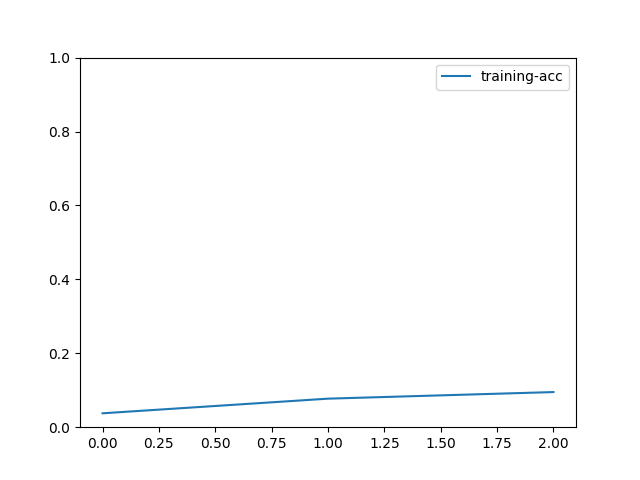
输出
[Epoch 0] train=0.037624 loss=4.593155 time: 43.816577
[Epoch 1] train=0.077228 loss=4.329765 time: 42.983821
[Epoch 2] train=0.095050 loss=4.159773 time: 43.229185
您可以立即开始训练。
如果您想在更大的数据集(例如 Kinetics400)上使用更大的 3D 模型(例如 I3D),请随时阅读下一篇关于 Kinetics400 的教程。
参考文献
- Wang15
Limin Wang, Yuanjun Xiong, Zhe Wang, and Yu Qiao. “Towards Good Practices for Very Deep Two-Stream ConvNets.” arXiv preprint arXiv:1507.02159 (2015).
- Wang16
Limin Wang, Yuanjun Xiong, Zhe Wang, Yu Qiao, Dahua Lin, Xiaoou Tang and Luc Van Gool. “Temporal Segment Networks: Towards Good Practices for Deep Action Recognition.” In European Conference on Computer Vision (ECCV). 2016.
脚本总运行时间: ( 2 minutes 11.163 seconds)