注意

点击这里下载完整的示例代码

06. 在 PASCAL VOC 上端到端训练 Faster-RCNN¶

本教程将介绍 GluonCV 提供的 Faster-RCNN [Ren15] 目标检测模型的基本训练步骤。

具体来说，我们将展示如何通过堆叠 GluonCV 组件来构建一个最先进的 Faster-RCNN 模型。

强烈建议阅读原始论文 [Girshick14]、[Girshick15]、[Ren15] 以了解 Faster R-CNN 背后的思想。来自 [He16] 的附录和来自 [Lin17] 的实验细节也可能是有用的参考。

提示

您可以跳过本教程的其余部分，直接下载此脚本开始训练您的 Faster-RCNN 模型

下载 train_faster_rcnn.py

示例用法

在 GPU 0 上使用 Pascal VOC 训练默认的 resnet50_v1b 模型

python train_faster_rcnn.py --gpus 0

在 GPU 0,1,2,3 上训练 resnet50_v1b 模型

python train_faster_rcnn.py --gpus 0,1,2,3 --network resnet50_v1b

检查支持的参数

python train_faster_rcnn.py --help

提示

由于本教程中的许多内容与 04. 在 Pascal VOC 数据集上训练 SSD 非常相似，如果您觉得熟悉，可以跳过任何部分。

数据集¶

请首先阅读此准备 PASCAL VOC 数据集教程，在您的磁盘上设置 Pascal VOC 数据集。然后，我们就可以加载训练和验证图像了。

from gluoncv.data import VOCDetection

# typically we use 2007+2012 trainval splits for training data
train_dataset = VOCDetection(splits=[(2007, 'trainval'), (2012, 'trainval')])
# and use 2007 test as validation data
val_dataset = VOCDetection(splits=[(2007, 'test')])

print('Training images:', len(train_dataset))
print('Validation images:', len(val_dataset))

输出

Training images: 16551
Validation images: 4952

数据转换¶

我们可以从训练数据集中读取图像-标签对

train_image, train_label = train_dataset[6]
bboxes = train_label[:, :4]
cids = train_label[:, 4:5]
print('image:', train_image.shape)
print('bboxes:', bboxes.shape, 'class ids:', cids.shape)

输出

image: (375, 500, 3)
bboxes: (2, 4) class ids: (2, 1)

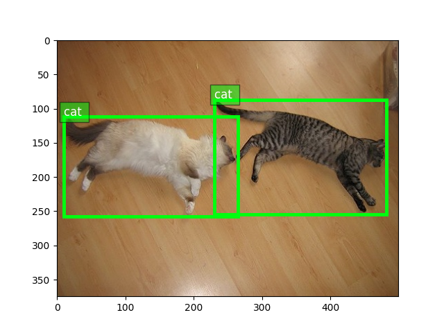
绘制图像以及边界框标签

from matplotlib import pyplot as plt
from gluoncv.utils import viz

ax = viz.plot_bbox(train_image.asnumpy(), bboxes, labels=cids, class_names=train_dataset.classes)
plt.show()

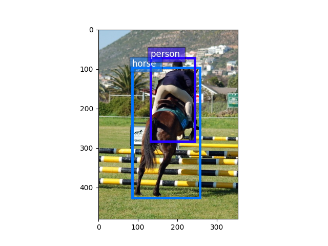
验证图像与训练图像非常相似，因为它们基本上是随机分割到不同集合的

val_image, val_label = val_dataset[6]
bboxes = val_label[:, :4]
cids = val_label[:, 4:5]
ax = viz.plot_bbox(val_image.asnumpy(), bboxes, labels=cids, class_names=train_dataset.classes)
plt.show()

对于 Faster-RCNN 网络，唯一的数据增强是水平翻转。

from gluoncv.data.transforms import presets
from gluoncv import utils
from mxnet import nd

short, max_size = 600, 1000  # resize image to short side 600 px, but keep maximum length within 1000
train_transform = presets.rcnn.FasterRCNNDefaultTrainTransform(short, max_size)
val_transform = presets.rcnn.FasterRCNNDefaultValTransform(short, max_size)

utils.random.seed(233)  # fix seed in this tutorial

我们对训练图像应用转换

train_image2, train_label2 = train_transform(train_image, train_label)
print('tensor shape:', train_image2.shape)
print('box and id shape:', train_label2.shape)

输出

tensor shape: (3, 600, 800)
box and id shape: (2, 6)

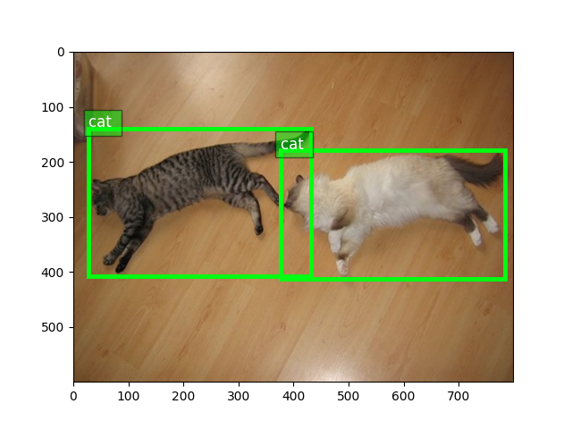
张量中的图像会失真，因为它们不再处于 (0, 255) 范围内。让我们将它们转换回来，以便我们可以清楚地看到它们。

train_image2 = train_image2.transpose((1, 2, 0)) * nd.array((0.229, 0.224, 0.225)) + nd.array(
    (0.485, 0.456, 0.406))
train_image2 = (train_image2 * 255).asnumpy().astype('uint8')
ax = viz.plot_bbox(train_image2, train_label2[:, :4],
                   labels=train_label2[:, 4:5],
                   class_names=train_dataset.classes)
plt.show()

数据加载器¶

训练期间，我们将多次迭代整个数据集。请记住，原始图像在输入到神经网络之前必须转换为张量（mxnet 使用 BCHW 格式）。

一个方便的数据加载器将非常便于我们应用不同的转换并将数据聚合成小批量。

由于 Faster-RCNN 处理具有各种纵横比和形状的原始图像，我们提供了一个 gluoncv.data.batchify.Append，它既不堆叠也不填充图像，而是返回列表。这样，返回的图像张量和标签具有自己的形状，不受同一批次中其余部分的影响。

from gluoncv.data.batchify import Tuple, Append, FasterRCNNTrainBatchify
from mxnet.gluon.data import DataLoader

batch_size = 2  # for tutorial, we use smaller batch-size
num_workers = 0  # you can make it larger(if your CPU has more cores) to accelerate data loading

# behavior of batchify_fn: stack images, and pad labels
batchify_fn = Tuple(Append(), Append())
train_loader = DataLoader(train_dataset.transform(train_transform), batch_size, shuffle=True,
                          batchify_fn=batchify_fn, last_batch='rollover', num_workers=num_workers)
val_loader = DataLoader(val_dataset.transform(val_transform), batch_size, shuffle=False,
                        batchify_fn=batchify_fn, last_batch='keep', num_workers=num_workers)

for ib, batch in enumerate(train_loader):
    if ib > 3:
        break
    print('data 0:', batch[0][0].shape, 'label 0:', batch[1][0].shape)
    print('data 1:', batch[0][1].shape, 'label 1:', batch[1][1].shape)

输出

data 0: (1, 3, 600, 800) label 0: (1, 5, 6)
data 1: (1, 3, 600, 901) label 1: (1, 9, 6)
data 0: (1, 3, 600, 800) label 0: (1, 2, 6)
data 1: (1, 3, 562, 1000) label 1: (1, 1, 6)
data 0: (1, 3, 600, 904) label 0: (1, 1, 6)
data 1: (1, 3, 600, 888) label 1: (1, 2, 6)
data 0: (1, 3, 600, 901) label 0: (1, 1, 6)
data 1: (1, 3, 600, 901) label 1: (1, 1, 6)

Faster-RCNN 网络¶

GluonCV 的 Faster-RCNN 实现是一个复合的 Gluon HybridBlock gluoncv.model_zoo.FasterRCNN。在结构上，Faster-RCNN 网络由基础特征提取网络、区域候选网络（包括其自身的锚点系统、候选区域生成器）、区域感知池化层、类别预测器和边界框偏移量预测器组成。

Gluon 模型库内置了一些 Faster-RCNN 网络，更多正在开发中。您只需一行简单的代码即可加载您喜欢的模型

提示

为了避免在本教程中下载模型，我们将 pretrained_base=False 设置为 False，实际中我们通常希望通过将 pretrained_base=True 设置为 True 来加载 ImageNet 预训练模型。

from gluoncv import model_zoo

net = model_zoo.get_model('faster_rcnn_resnet50_v1b_voc', pretrained_base=False)
print(net)

输出

FasterRCNN(
  (features): HybridSequential(
    (0): Conv2D(None -> 64, kernel_size=(7, 7), stride=(2, 2), padding=(3, 3), bias=False)
    (1): BatchNorm(axis=1, eps=1e-05, momentum=0.9, fix_gamma=False, use_global_stats=True, in_channels=64)
    (2): Activation(relu)
    (3): MaxPool2D(size=(3, 3), stride=(2, 2), padding=(1, 1), ceil_mode=False, global_pool=False, pool_type=max, layout=NCHW)
    (4): HybridSequential(
      (0): BottleneckV1b(
        (conv1): Conv2D(None -> 64, kernel_size=(1, 1), stride=(1, 1), bias=False)
        (bn1): BatchNorm(axis=1, eps=1e-05, momentum=0.9, fix_gamma=False, use_global_stats=True, in_channels=64)
        (relu1): Activation(relu)
        (conv2): Conv2D(None -> 64, kernel_size=(3, 3), stride=(1, 1), padding=(1, 1), bias=False)
        (bn2): BatchNorm(axis=1, eps=1e-05, momentum=0.9, fix_gamma=False, use_global_stats=True, in_channels=64)
        (relu2): Activation(relu)
        (conv3): Conv2D(None -> 256, kernel_size=(1, 1), stride=(1, 1), bias=False)
        (bn3): BatchNorm(axis=1, eps=1e-05, momentum=0.9, fix_gamma=False, use_global_stats=True, in_channels=256)
        (relu3): Activation(relu)
        (downsample): HybridSequential(
          (0): Conv2D(None -> 256, kernel_size=(1, 1), stride=(1, 1), bias=False)
          (1): BatchNorm(axis=1, eps=1e-05, momentum=0.9, fix_gamma=False, use_global_stats=True, in_channels=256)
        )
      )
      (1): BottleneckV1b(
        (conv1): Conv2D(None -> 64, kernel_size=(1, 1), stride=(1, 1), bias=False)
        (bn1): BatchNorm(axis=1, eps=1e-05, momentum=0.9, fix_gamma=False, use_global_stats=True, in_channels=64)
        (relu1): Activation(relu)
        (conv2): Conv2D(None -> 64, kernel_size=(3, 3), stride=(1, 1), padding=(1, 1), bias=False)
        (bn2): BatchNorm(axis=1, eps=1e-05, momentum=0.9, fix_gamma=False, use_global_stats=True, in_channels=64)
        (relu2): Activation(relu)
        (conv3): Conv2D(None -> 256, kernel_size=(1, 1), stride=(1, 1), bias=False)
        (bn3): BatchNorm(axis=1, eps=1e-05, momentum=0.9, fix_gamma=False, use_global_stats=True, in_channels=256)
        (relu3): Activation(relu)
      )
      (2): BottleneckV1b(
        (conv1): Conv2D(None -> 64, kernel_size=(1, 1), stride=(1, 1), bias=False)
        (bn1): BatchNorm(axis=1, eps=1e-05, momentum=0.9, fix_gamma=False, use_global_stats=True, in_channels=64)
        (relu1): Activation(relu)
        (conv2): Conv2D(None -> 64, kernel_size=(3, 3), stride=(1, 1), padding=(1, 1), bias=False)
        (bn2): BatchNorm(axis=1, eps=1e-05, momentum=0.9, fix_gamma=False, use_global_stats=True, in_channels=64)
        (relu2): Activation(relu)
        (conv3): Conv2D(None -> 256, kernel_size=(1, 1), stride=(1, 1), bias=False)
        (bn3): BatchNorm(axis=1, eps=1e-05, momentum=0.9, fix_gamma=False, use_global_stats=True, in_channels=256)
        (relu3): Activation(relu)
      )
    )
    (5): HybridSequential(
      (0): BottleneckV1b(
        (conv1): Conv2D(None -> 128, kernel_size=(1, 1), stride=(1, 1), bias=False)
        (bn1): BatchNorm(axis=1, eps=1e-05, momentum=0.9, fix_gamma=False, use_global_stats=True, in_channels=128)
        (relu1): Activation(relu)
        (conv2): Conv2D(None -> 128, kernel_size=(3, 3), stride=(2, 2), padding=(1, 1), bias=False)
        (bn2): BatchNorm(axis=1, eps=1e-05, momentum=0.9, fix_gamma=False, use_global_stats=True, in_channels=128)
        (relu2): Activation(relu)
        (conv3): Conv2D(None -> 512, kernel_size=(1, 1), stride=(1, 1), bias=False)
        (bn3): BatchNorm(axis=1, eps=1e-05, momentum=0.9, fix_gamma=False, use_global_stats=True, in_channels=512)
        (relu3): Activation(relu)
        (downsample): HybridSequential(
          (0): Conv2D(None -> 512, kernel_size=(1, 1), stride=(2, 2), bias=False)
          (1): BatchNorm(axis=1, eps=1e-05, momentum=0.9, fix_gamma=False, use_global_stats=True, in_channels=512)
        )
      )
      (1): BottleneckV1b(
        (conv1): Conv2D(None -> 128, kernel_size=(1, 1), stride=(1, 1), bias=False)
        (bn1): BatchNorm(axis=1, eps=1e-05, momentum=0.9, fix_gamma=False, use_global_stats=True, in_channels=128)
        (relu1): Activation(relu)
        (conv2): Conv2D(None -> 128, kernel_size=(3, 3), stride=(1, 1), padding=(1, 1), bias=False)
        (bn2): BatchNorm(axis=1, eps=1e-05, momentum=0.9, fix_gamma=False, use_global_stats=True, in_channels=128)
        (relu2): Activation(relu)
        (conv3): Conv2D(None -> 512, kernel_size=(1, 1), stride=(1, 1), bias=False)
        (bn3): BatchNorm(axis=1, eps=1e-05, momentum=0.9, fix_gamma=False, use_global_stats=True, in_channels=512)
        (relu3): Activation(relu)
      )
      (2): BottleneckV1b(
        (conv1): Conv2D(None -> 128, kernel_size=(1, 1), stride=(1, 1), bias=False)
        (bn1): BatchNorm(axis=1, eps=1e-05, momentum=0.9, fix_gamma=False, use_global_stats=True, in_channels=128)
        (relu1): Activation(relu)
        (conv2): Conv2D(None -> 128, kernel_size=(3, 3), stride=(1, 1), padding=(1, 1), bias=False)
        (bn2): BatchNorm(axis=1, eps=1e-05, momentum=0.9, fix_gamma=False, use_global_stats=True, in_channels=128)
        (relu2): Activation(relu)
        (conv3): Conv2D(None -> 512, kernel_size=(1, 1), stride=(1, 1), bias=False)
        (bn3): BatchNorm(axis=1, eps=1e-05, momentum=0.9, fix_gamma=False, use_global_stats=True, in_channels=512)
        (relu3): Activation(relu)
      )
      (3): BottleneckV1b(
        (conv1): Conv2D(None -> 128, kernel_size=(1, 1), stride=(1, 1), bias=False)
        (bn1): BatchNorm(axis=1, eps=1e-05, momentum=0.9, fix_gamma=False, use_global_stats=True, in_channels=128)
        (relu1): Activation(relu)
        (conv2): Conv2D(None -> 128, kernel_size=(3, 3), stride=(1, 1), padding=(1, 1), bias=False)
        (bn2): BatchNorm(axis=1, eps=1e-05, momentum=0.9, fix_gamma=False, use_global_stats=True, in_channels=128)
        (relu2): Activation(relu)
        (conv3): Conv2D(None -> 512, kernel_size=(1, 1), stride=(1, 1), bias=False)
        (bn3): BatchNorm(axis=1, eps=1e-05, momentum=0.9, fix_gamma=False, use_global_stats=True, in_channels=512)
        (relu3): Activation(relu)
      )
    )
    (6): HybridSequential(
      (0): BottleneckV1b(
        (conv1): Conv2D(None -> 256, kernel_size=(1, 1), stride=(1, 1), bias=False)
        (bn1): BatchNorm(axis=1, eps=1e-05, momentum=0.9, fix_gamma=False, use_global_stats=True, in_channels=256)
        (relu1): Activation(relu)
        (conv2): Conv2D(None -> 256, kernel_size=(3, 3), stride=(2, 2), padding=(1, 1), bias=False)
        (bn2): BatchNorm(axis=1, eps=1e-05, momentum=0.9, fix_gamma=False, use_global_stats=True, in_channels=256)
        (relu2): Activation(relu)
        (conv3): Conv2D(None -> 1024, kernel_size=(1, 1), stride=(1, 1), bias=False)
        (bn3): BatchNorm(axis=1, eps=1e-05, momentum=0.9, fix_gamma=False, use_global_stats=True, in_channels=1024)
        (relu3): Activation(relu)
        (downsample): HybridSequential(
          (0): Conv2D(None -> 1024, kernel_size=(1, 1), stride=(2, 2), bias=False)
          (1): BatchNorm(axis=1, eps=1e-05, momentum=0.9, fix_gamma=False, use_global_stats=True, in_channels=1024)
        )
      )
      (1): BottleneckV1b(
        (conv1): Conv2D(None -> 256, kernel_size=(1, 1), stride=(1, 1), bias=False)
        (bn1): BatchNorm(axis=1, eps=1e-05, momentum=0.9, fix_gamma=False, use_global_stats=True, in_channels=256)
        (relu1): Activation(relu)
        (conv2): Conv2D(None -> 256, kernel_size=(3, 3), stride=(1, 1), padding=(1, 1), bias=False)
        (bn2): BatchNorm(axis=1, eps=1e-05, momentum=0.9, fix_gamma=False, use_global_stats=True, in_channels=256)
        (relu2): Activation(relu)
        (conv3): Conv2D(None -> 1024, kernel_size=(1, 1), stride=(1, 1), bias=False)
        (bn3): BatchNorm(axis=1, eps=1e-05, momentum=0.9, fix_gamma=False, use_global_stats=True, in_channels=1024)
        (relu3): Activation(relu)
      )
      (2): BottleneckV1b(
        (conv1): Conv2D(None -> 256, kernel_size=(1, 1), stride=(1, 1), bias=False)
        (bn1): BatchNorm(axis=1, eps=1e-05, momentum=0.9, fix_gamma=False, use_global_stats=True, in_channels=256)
        (relu1): Activation(relu)
        (conv2): Conv2D(None -> 256, kernel_size=(3, 3), stride=(1, 1), padding=(1, 1), bias=False)
        (bn2): BatchNorm(axis=1, eps=1e-05, momentum=0.9, fix_gamma=False, use_global_stats=True, in_channels=256)
        (relu2): Activation(relu)
        (conv3): Conv2D(None -> 1024, kernel_size=(1, 1), stride=(1, 1), bias=False)
        (bn3): BatchNorm(axis=1, eps=1e-05, momentum=0.9, fix_gamma=False, use_global_stats=True, in_channels=1024)
        (relu3): Activation(relu)
      )
      (3): BottleneckV1b(
        (conv1): Conv2D(None -> 256, kernel_size=(1, 1), stride=(1, 1), bias=False)
        (bn1): BatchNorm(axis=1, eps=1e-05, momentum=0.9, fix_gamma=False, use_global_stats=True, in_channels=256)
        (relu1): Activation(relu)
        (conv2): Conv2D(None -> 256, kernel_size=(3, 3), stride=(1, 1), padding=(1, 1), bias=False)
        (bn2): BatchNorm(axis=1, eps=1e-05, momentum=0.9, fix_gamma=False, use_global_stats=True, in_channels=256)
        (relu2): Activation(relu)
        (conv3): Conv2D(None -> 1024, kernel_size=(1, 1), stride=(1, 1), bias=False)
        (bn3): BatchNorm(axis=1, eps=1e-05, momentum=0.9, fix_gamma=False, use_global_stats=True, in_channels=1024)
        (relu3): Activation(relu)
      )
      (4): BottleneckV1b(
        (conv1): Conv2D(None -> 256, kernel_size=(1, 1), stride=(1, 1), bias=False)
        (bn1): BatchNorm(axis=1, eps=1e-05, momentum=0.9, fix_gamma=False, use_global_stats=True, in_channels=256)
        (relu1): Activation(relu)
        (conv2): Conv2D(None -> 256, kernel_size=(3, 3), stride=(1, 1), padding=(1, 1), bias=False)
        (bn2): BatchNorm(axis=1, eps=1e-05, momentum=0.9, fix_gamma=False, use_global_stats=True, in_channels=256)
        (relu2): Activation(relu)
        (conv3): Conv2D(None -> 1024, kernel_size=(1, 1), stride=(1, 1), bias=False)
        (bn3): BatchNorm(axis=1, eps=1e-05, momentum=0.9, fix_gamma=False, use_global_stats=True, in_channels=1024)
        (relu3): Activation(relu)
      )
      (5): BottleneckV1b(
        (conv1): Conv2D(None -> 256, kernel_size=(1, 1), stride=(1, 1), bias=False)
        (bn1): BatchNorm(axis=1, eps=1e-05, momentum=0.9, fix_gamma=False, use_global_stats=True, in_channels=256)
        (relu1): Activation(relu)
        (conv2): Conv2D(None -> 256, kernel_size=(3, 3), stride=(1, 1), padding=(1, 1), bias=False)
        (bn2): BatchNorm(axis=1, eps=1e-05, momentum=0.9, fix_gamma=False, use_global_stats=True, in_channels=256)
        (relu2): Activation(relu)
        (conv3): Conv2D(None -> 1024, kernel_size=(1, 1), stride=(1, 1), bias=False)
        (bn3): BatchNorm(axis=1, eps=1e-05, momentum=0.9, fix_gamma=False, use_global_stats=True, in_channels=1024)
        (relu3): Activation(relu)
      )
    )
  )
  (top_features): HybridSequential(
    (0): HybridSequential(
      (0): BottleneckV1b(
        (conv1): Conv2D(None -> 512, kernel_size=(1, 1), stride=(1, 1), bias=False)
        (bn1): BatchNorm(axis=1, eps=1e-05, momentum=0.9, fix_gamma=False, use_global_stats=True, in_channels=512)
        (relu1): Activation(relu)
        (conv2): Conv2D(None -> 512, kernel_size=(3, 3), stride=(2, 2), padding=(1, 1), bias=False)
        (bn2): BatchNorm(axis=1, eps=1e-05, momentum=0.9, fix_gamma=False, use_global_stats=True, in_channels=512)
        (relu2): Activation(relu)
        (conv3): Conv2D(None -> 2048, kernel_size=(1, 1), stride=(1, 1), bias=False)
        (bn3): BatchNorm(axis=1, eps=1e-05, momentum=0.9, fix_gamma=False, use_global_stats=True, in_channels=2048)
        (relu3): Activation(relu)
        (downsample): HybridSequential(
          (0): Conv2D(None -> 2048, kernel_size=(1, 1), stride=(2, 2), bias=False)
          (1): BatchNorm(axis=1, eps=1e-05, momentum=0.9, fix_gamma=False, use_global_stats=True, in_channels=2048)
        )
      )
      (1): BottleneckV1b(
        (conv1): Conv2D(None -> 512, kernel_size=(1, 1), stride=(1, 1), bias=False)
        (bn1): BatchNorm(axis=1, eps=1e-05, momentum=0.9, fix_gamma=False, use_global_stats=True, in_channels=512)
        (relu1): Activation(relu)
        (conv2): Conv2D(None -> 512, kernel_size=(3, 3), stride=(1, 1), padding=(1, 1), bias=False)
        (bn2): BatchNorm(axis=1, eps=1e-05, momentum=0.9, fix_gamma=False, use_global_stats=True, in_channels=512)
        (relu2): Activation(relu)
        (conv3): Conv2D(None -> 2048, kernel_size=(1, 1), stride=(1, 1), bias=False)
        (bn3): BatchNorm(axis=1, eps=1e-05, momentum=0.9, fix_gamma=False, use_global_stats=True, in_channels=2048)
        (relu3): Activation(relu)
      )
      (2): BottleneckV1b(
        (conv1): Conv2D(None -> 512, kernel_size=(1, 1), stride=(1, 1), bias=False)
        (bn1): BatchNorm(axis=1, eps=1e-05, momentum=0.9, fix_gamma=False, use_global_stats=True, in_channels=512)
        (relu1): Activation(relu)
        (conv2): Conv2D(None -> 512, kernel_size=(3, 3), stride=(1, 1), padding=(1, 1), bias=False)
        (bn2): BatchNorm(axis=1, eps=1e-05, momentum=0.9, fix_gamma=False, use_global_stats=True, in_channels=512)
        (relu2): Activation(relu)
        (conv3): Conv2D(None -> 2048, kernel_size=(1, 1), stride=(1, 1), bias=False)
        (bn3): BatchNorm(axis=1, eps=1e-05, momentum=0.9, fix_gamma=False, use_global_stats=True, in_channels=2048)
        (relu3): Activation(relu)
      )
    )
  )
  (class_predictor): Dense(None -> 21, linear)
  (box_predictor): Dense(None -> 80, linear)
  (cls_decoder): MultiPerClassDecoder(

  )
  (box_decoder): NormalizedBoxCenterDecoder(
    (corner_to_center): BBoxCornerToCenter(

    )
  )
  (rpn): RPN(
    (anchor_generator): RPNAnchorGenerator(

    )
    (conv1): HybridSequential(
      (0): Conv2D(None -> 1024, kernel_size=(3, 3), stride=(1, 1), padding=(1, 1))
      (1): Activation(relu)
    )
    (score): Conv2D(None -> 15, kernel_size=(1, 1), stride=(1, 1))
    (loc): Conv2D(None -> 60, kernel_size=(1, 1), stride=(1, 1))
    (region_proposer): RPNProposal(
      (_box_to_center): BBoxCornerToCenter(

      )
      (_box_decoder): NormalizedBoxCenterDecoder(
        (corner_to_center): BBoxCornerToCenter(

        )
      )
      (_clipper): BBoxClipToImage(

      )
    )
  )
  (sampler): RCNNTargetSampler(

  )
)

Faster-RCNN 网络可以使用图像张量调用

import mxnet as mx

x = mx.nd.zeros(shape=(1, 3, 600, 800))
net.initialize()
cids, scores, bboxes = net(x)

Faster-RCNN 返回三个值，其中 cids 是类别标签，scores 是每个预测的置信度得分，以及 bboxes 是相应边界框的绝对坐标。

Faster-RCNN 网络在训练模式下的行为不同

from mxnet import autograd

with autograd.train_mode():
    # this time we need ground-truth to generate high quality roi proposals during training
    gt_box = mx.nd.zeros(shape=(1, 1, 4))
    gt_label = mx.nd.zeros(shape=(1, 1, 1))
    cls_pred, box_pred, roi, samples, matches, rpn_score, rpn_box, anchors, cls_targets, \
        box_targets, box_masks, _ = net(x, gt_box, gt_label)

在训练模式下，Faster-RCNN 返回许多中间值，这些值是进行端到端训练所必需的，其中 cls_preds 是 softmax 之前的类别预测，box_preds 是与候选区域一一对应的边界框偏移量，roi 是候选区域，samples 和 matches 是 RPN 锚点的采样/匹配结果。rpn_score 和 rpn_box 是 RPN 卷积层的原始输出。而 anchors 是相应锚框的绝对坐标。

训练损失¶

端到端 Faster-RCNN 训练涉及四种损失。

# the loss to penalize incorrect foreground/background prediction
rpn_cls_loss = mx.gluon.loss.SigmoidBinaryCrossEntropyLoss(from_sigmoid=False)
# the loss to penalize inaccurate anchor boxes
rpn_box_loss = mx.gluon.loss.HuberLoss(rho=1 / 9.)  # == smoothl1
# the loss to penalize incorrect classification prediction.
rcnn_cls_loss = mx.gluon.loss.SoftmaxCrossEntropyLoss()
# and finally the loss to penalize inaccurate proposals
rcnn_box_loss = mx.gluon.loss.HuberLoss()  # == smoothl1

RPN 训练目标¶

为了加快训练速度，我们让 CPU 预先计算 RPN 训练目标。当您的 CPU 性能强大并且您可以使用 -j num_workers 来利用多核 CPU 时，这尤其有用。

如果我们向训练转换函数提供网络，它将计算训练目标

train_transform = presets.rcnn.FasterRCNNDefaultTrainTransform(short, max_size, net)
# Return images, labels, rpn_cls_targets, rpn_box_targets, rpn_box_masks loosely
batchify_fn = FasterRCNNTrainBatchify(net)
# For the next part, we only use batch size 1
batch_size = 1
train_loader = DataLoader(train_dataset.transform(train_transform), batch_size, shuffle=True,
                          batchify_fn=batchify_fn, last_batch='rollover', num_workers=num_workers)

这次我们可以看到数据加载器实际上正在为我们返回训练目标。然后，很自然地就可以使用 Trainer 进行 gluon 训练循环并让它更新权重。

for ib, batch in enumerate(train_loader):
    if ib > 0:
        break
    with autograd.train_mode():
        for data, label, rpn_cls_targets, rpn_box_targets, rpn_box_masks in zip(*batch):
            label = label.expand_dims(0)
            gt_label = label[:, :, 4:5]
            gt_box = label[:, :, :4]
            print('data:', data.shape)
            # box and class labels
            print('box:', gt_box.shape)
            print('label:', gt_label.shape)
            # -1 marks ignored label
            print('rpn cls label:', rpn_cls_targets.shape)
            # mask out ignored box label
            print('rpn box label:', rpn_box_targets.shape)
            print('rpn box mask:', rpn_box_masks.shape)

输出

data: (3, 600, 800)
box: (1, 6, 4)
label: (1, 6, 1)
rpn cls label: (1, 28500)
rpn box label: (1, 28500, 4)
rpn box mask: (1, 28500, 4)

RCNN 训练目标¶

RCNN 目标是使用存储的目标生成器从中间输出生成的。

for ib, batch in enumerate(train_loader):
    if ib > 0:
        break
    with autograd.train_mode():
        for data, label, rpn_cls_targets, rpn_box_targets, rpn_box_masks in zip(*batch):
            label = label.expand_dims(0)
            gt_label = label[:, :, 4:5]
            gt_box = label[:, :, :4]
            # network forward
            cls_pred, box_pred, roi, samples, matches, rpn_score, rpn_box, anchors, cls_targets, \
                box_targets, box_masks, _ = net(data.expand_dims(0), gt_box, gt_label)

            print('data:', data.shape)
            # box and class labels
            print('box:', gt_box.shape)
            print('label:', gt_label.shape)
            # rcnn does not have ignored label
            print('rcnn cls label:', cls_targets.shape)
            # mask out ignored box label
            print('rcnn box label:', box_targets.shape)
            print('rcnn box mask:', box_masks.shape)

输出

data: (3, 600, 800)
box: (1, 2, 4)
label: (1, 2, 1)
rcnn cls label: (1, 128)
rcnn box label: (1, 32, 20, 4)
rcnn box mask: (1, 32, 20, 4)

训练循环¶

定义好损失函数并生成训练目标后，我们就可以编写训练循环了。

for ib, batch in enumerate(train_loader):
    if ib > 0:
        break
    with autograd.record():
        for data, label, rpn_cls_targets, rpn_box_targets, rpn_box_masks in zip(*batch):
            label = label.expand_dims(0)
            gt_label = label[:, :, 4:5]
            gt_box = label[:, :, :4]
            # network forward
            cls_preds, box_preds, roi, samples, matches, rpn_score, rpn_box, anchors, cls_targets, \
                box_targets, box_masks, _ = net(data.expand_dims(0), gt_box, gt_label)

            # losses of rpn
            rpn_score = rpn_score.squeeze(axis=-1)
            num_rpn_pos = (rpn_cls_targets >= 0).sum()
            rpn_loss1 = rpn_cls_loss(rpn_score, rpn_cls_targets,
                                     rpn_cls_targets >= 0) * rpn_cls_targets.size / num_rpn_pos
            rpn_loss2 = rpn_box_loss(rpn_box, rpn_box_targets,
                                     rpn_box_masks) * rpn_box.size / num_rpn_pos

            # losses of rcnn
            num_rcnn_pos = (cls_targets >= 0).sum()
            rcnn_loss1 = rcnn_cls_loss(cls_preds, cls_targets,
                                       cls_targets >= 0) * cls_targets.size / cls_targets.shape[
                             0] / num_rcnn_pos
            rcnn_loss2 = rcnn_box_loss(box_preds, box_targets, box_masks) * box_preds.size / \
                         box_preds.shape[0] / num_rcnn_pos

        # some standard gluon training steps:
        # autograd.backward([rpn_loss1, rpn_loss2, rcnn_loss1, rcnn_loss2])
        # trainer.step(batch_size)

提示

请查看完整的 训练脚本 以获取完整实现。

参考文献¶

Girshick14: Ross Girshick, Jeff Donahue, Trevor Darrell 和 Jitendra Malik。用于精确目标检测和语义分割的丰富特征层次结构。CVPR 2014。
Girshick15: Ross Girshick。快速 {R-CNN}。ICCV 2015。
Ren15(1,2): Shaoqing Ren, Kaiming He, Ross Girshick 和 Jian Sun。Faster {R-CNN}：使用区域候选网络实现实时目标检测。NIPS 2015。
He16: Kaiming He, Xiangyu Zhang, Shaoqing Ren 和 Jian Sun。用于图像识别的深度残差学习。CVPR 2016。
Lin17: Tsung-Yi Lin, Piotr Dollár, Ross Girshick, Kaiming He, Bharath Hariharan 和 Serge Belongie。用于目标检测的特征金字塔网络。CVPR 2017。

脚本总运行时间： ( 0 分 28.802 秒)

由 Sphinx-Gallery 生成的图库