注意
点击 这里 下载完整的示例代码
5. 在 ImageNet 上训练自己的模型
ImageNet 是图像分类领域最著名的数据集。自发布以来,大多数推动图像分类技术进步的研究都是基于该数据集。
尽管有许多可用的模型,但从零开始在 ImageNet 上训练一个最先进的模型仍然是一项不简单的任务。在本教程中,我们将流畅地指导您完成在 ImageNet 上训练模型的过程。
注意
由于实际训练非常消耗资源,本教程中我们不会实际执行代码块。
先决条件
专业知识
我们假设读者对 Gluon 有基本的了解,建议您从 Gluon 速成课 开始学习。
此外,我们假设读者已经学习了之前的 CIFAR10 训练 和 ImageNet 示例 教程。
数据准备
与 CIFAR10 不同,我们需要手动准备数据。如果您还没有这样做,请学习我们的 准备 ImageNet 数据 教程。
硬件
在包含一百多万张图像的数据集上训练深度学习模型非常耗费资源。两个主要瓶颈是张量计算和数据 I/O。
对于张量计算,建议使用 GPU,最好是高端 GPU。使用多块 GPU 可以进一步缩短训练时间。
对于数据 I/O,我们推荐使用快速 CPU 和 SSD 硬盘。数据加载可以从多个 CPU 线程和快速 SSD 硬盘中大大受益。请注意,压缩和提取的 ImageNet 数据总共可能占用约 300GB 的磁盘空间,因此需要至少 300GB 的 SSD 硬盘。
网络结构
准备好了吗?开始吧!
首先,将必要的库导入到 python 中。
import argparse, time

import numpy as np
import mxnet as mx

from mxnet import gluon, nd
from mxnet import autograd as ag
from mxnet.gluon import nn

from gluoncv.model_zoo import get_model
from gluoncv.utils import makedirs, TrainingHistory
在本教程中,我们使用 ResNet50_v2,这是一个在预测精度和计算成本之间达到平衡的网络。
# number of GPUs to use
num_gpus = 4
ctx = [mx.gpu(i) for i in range(num_gpus)]

# Get the model ResNet50_v2, with 10 output classes
net = get_model('ResNet50_v2', classes=1000)
net.initialize(mx.init.MSRAPrelu(), ctx = ctx)
请注意,我们在此用于 ImageNet 的 ResNet 模型在结构上与我们用于训练 CIFAR10 的模型不同。详细信息请参考原始论文或 GluonCV 代码库。
使用 ImageRecordIter 进行数据增强
当使用多块 GPU 训练小型网络时,数据 I/O 可能成为性能瓶颈。除了 gluon 的数据加载器,我们推荐使用 ImageRecordIter 接口从记录文件中加载和处理数据。有关记录文件的更多信息,请参考我们的教程。
数据增强对于取得好结果至关重要。我们可以在 ImageRecordIter 中设置相关参数。
jitter_param = 0.4
lighting_param = 0.1
mean_rgb = [123.68, 116.779, 103.939]
std_rgb = [58.393, 57.12, 57.375]

train_data = mx.io.ImageRecordIter(
    path_imgrec         = '~/.mxnet/datasets/imagenet/rec/train.rec',
    path_imgidx         = '~/.mxnet/datasets/imagenet/rec/train.idx',
    preprocess_threads  = 32,
    shuffle             = True,
    batch_size          = 256,

    data_shape          = (3, 224, 224),
    mean_r              = mean_rgb[0],
    mean_g              = mean_rgb[1],
    mean_b              = mean_rgb[2],
    std_r               = std_rgb[0],
    std_g               = std_rgb[1],
    std_b               = std_rgb[2],
    rand_mirror         = True,
    random_resized_crop = True,
    max_aspect_ratio    = 4. / 3.,
    min_aspect_ratio    = 3. / 4.,
    max_random_area     = 1,
    min_random_area     = 0.08,
    brightness          = jitter_param,
    saturation          = jitter_param,
    contrast            = jitter_param,
    pca_noise           = lighting_param,
)
由于 ImageNet 图像的分辨率和质量远高于 CIFAR10,我们可以裁剪更大的图像(224x224)作为模型的输入。
对于预测,我们仍然需要确定性的结果。读取函数是
val_data = mx.io.ImageRecordIter(
    path_imgrec         = '~/.mxnet/datasets/imagenet/rec/val.rec',
    path_imgidx         = '~/.mxnet/datasets/imagenet/rec/val.idx',
    preprocess_threads  = 32,
    shuffle             = False,
    batch_size          = 256,

    resize              = 256,
    data_shape          = (3, 224, 224),
    mean_r              = mean_rgb[0],
    mean_g              = mean_rgb[1],
    mean_b              = mean_rgb[2],
    std_r               = std_rgb[0],
    std_g               = std_rgb[1],
    std_b               = std_rgb[2],
)
保持归一化一致性非常重要,因为训练好的模型仅在来自相同分布的测试数据上表现良好。
上面的代码作为数据加载器工作,因此我们稍后可以直接将它们插入到训练循环中。
请注意,我们将 batch_size=256 设置为 4 块 GPU 上的总批量大小。这可能不适用于显存小于 12GB 的 GPU。请根据您的具体配置调整该值。
如果您使用我们的脚本准备数据,路径 '~/.mxnet/datasets/imagenet/rec' 是默认路径。
优化器、损失函数和评估指标
优化器是在训练过程中改进模型的方法。我们使用流行的 Nesterov 加速梯度下降算法。
# Learning rate decay factor
lr_decay = 0.1
# Epochs where learning rate decays
lr_decay_epoch = [30, 60, 90, np.inf]

# Nesterov accelerated gradient descent
optimizer = 'nag'
# Set parameters
optimizer_params = {'learning_rate': 0.1, 'wd': 0.0001, 'momentum': 0.9}

# Define our trainer for net
trainer = gluon.Trainer(net.collect_params(), optimizer, optimizer_params)
对于分类任务,我们通常使用 softmax 交叉熵作为损失函数。
loss_fn = gluon.loss.SoftmaxCrossEntropyLoss()
对于 1000 个类别,模型可能并非总是将正确答案排在最高位置。除了 Top-1 准确率,我们还考虑 Top-5 准确率作为衡量模型性能好坏的指标。
在每个 epoch 结束时,我们记录并打印评估指标得分。
acc_top1 = mx.metric.Accuracy()
acc_top5 = mx.metric.TopKAccuracy(5)
train_history = TrainingHistory(['training-top1-err', 'training-top5-err',
                                 'validation-top1-err', 'validation-top5-err'])
验证
在每个训练 epoch 结束时,我们在验证数据集上评估模型,并报告 Top-1 和 Top-5 错误率。
def test(ctx, val_data):
    acc_top1_val = mx.metric.Accuracy()
    acc_top5_val = mx.metric.TopKAccuracy(5)
    for i, batch in enumerate(val_data):
        data = gluon.utils.split_and_load(batch.data[0], ctx_list=ctx, batch_axis=0)
        label = gluon.utils.split_and_load(batch.label[0], ctx_list=ctx, batch_axis=0)
        outputs = [net(X) for X in data]
        acc_top1_val.update(label, outputs)
        acc_top5_val.update(label, outputs)

    _, top1 = acc_top1_val.get()
    _, top5 = acc_top5_val.get()
    return (1 - top1, 1 - top5)
训练
完成所有准备工作后,我们终于可以开始训练了!以下是主要的训练循环
epochs = 120
lr_decay_count = 0
log_interval = 50

for epoch in range(epochs):
    tic = time.time()
    btic = time.time()
    acc_top1.reset()
    acc_top5.reset()

    if lr_decay_period == 0 and epoch == lr_decay_epoch[lr_decay_count]:
        trainer.set_learning_rate(trainer.learning_rate*lr_decay)
        lr_decay_count += 1

    for i, batch in enumerate(train_data):
        data = gluon.utils.split_and_load(batch.data[0], ctx_list=ctx, batch_axis=0)
        label = gluon.utils.split_and_load(batch.label[0], ctx_list=ctx, batch_axis=0)
        with ag.record():
            outputs = [net(X) for X in data]
            loss = [L(yhat, y) for yhat, y in zip(outputs, label)]
        ag.backward(loss)
        trainer.step(batch_size)
        acc_top1.update(label, outputs)
        acc_top5.update(label, outputs)
        if log_interval and not (i + 1) % log_interval:
            _, top1 = acc_top1.get()
            _, top5 = acc_top5.get()
            err_top1, err_top5 = (1-top1, 1-top5)
            print('Epoch[%d] Batch [%d]     Speed: %f samples/sec   top1-err=%f     top5-err=%f'%(
                      epoch, i, batch_size*opt.log_interval/(time.time()-btic), err_top1, err_top5))
            btic = time.time()

    _, top1 = acc_top1.get()
    _, top5 = acc_top5.get()
    err_top1, err_top5 = (1-top1, 1-top5)

    err_top1_val, err_top5_val = test(ctx, val_data)
    train_history.update([err_top1, err_top5, err_top1_val, err_top5_val])

    print('[Epoch %d] training: err-top1=%f err-top5=%f'%(epoch, err_top1, err_top5))
    print('[Epoch %d] time cost: %f'%(epoch, time.time()-tic))
    print('[Epoch %d] validation: err-top1=%f err-top5=%f'%(epoch, err_top1_val, err_top5_val))
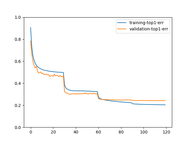
我们可以用以下方法绘制 Top-1 错误率
train_history.plot(['training-top1-err', 'validation-top1-err'])
如果您用 epochs=120 训练模型,绘制的图可能看起来像