1. 使用预训练的Simple Pose人体姿态估计模型进行预测

本文介绍如何通过几行代码使用预训练的Simple Pose模型。

首先导入必要的库

from matplotlib import pyplot as plt
from gluoncv import model_zoo, data, utils
from gluoncv.data.transforms.pose import detector_to_simple_pose, heatmap_to_coord

加载预训练模型

我们获取一个在MS COCO数据集上以256x192输入图像大小训练的Simple Pose模型。我们选择使用ResNet-18 V1b作为基础模型的那个。通过指定pretrained=True，如果需要，它将自动从模型库下载模型。更多预训练模型，请参考模型库。

请注意，Simple Pose模型采用自上而下（top-down）的策略，从目标检测模型检测到的边界框中估计人体姿态。

detector = model_zoo.get_model('yolo3_mobilenet1.0_coco', pretrained=True)
pose_net = model_zoo.get_model('simple_pose_resnet18_v1b', pretrained=True)

# Note that we can reset the classes of the detector to only include
# human, so that the NMS process is faster.

detector.reset_class(["person"], reuse_weights=['person'])

输出

Downloading /root/.mxnet/models/yolo3_mobilenet1.0_coco-66dbbae6.zip from https://apache-mxnet.s3-accelerate.dualstack.amazonaws.com/gluon/models/yolo3_mobilenet1.0_coco-66dbbae6.zip...

  0%|          | 0/88992 [00:00<?, ?KB/s]
  1%|          | 642/88992 [00:00<00:17, 5145.99KB/s]
  4%|3         | 3288/88992 [00:00<00:05, 14572.57KB/s]
 12%|#1        | 10253/88992 [00:00<00:02, 36718.39KB/s]
 19%|#9        | 17291/88992 [00:00<00:01, 48998.77KB/s]
 29%|##8       | 25640/88992 [00:00<00:01, 60811.68KB/s]
 37%|###7      | 32979/88992 [00:00<00:00, 64943.31KB/s]
 46%|####5     | 40816/88992 [00:00<00:00, 68490.18KB/s]
 55%|#####5    | 48964/88992 [00:00<00:00, 72529.44KB/s]
 64%|######4   | 56985/88992 [00:00<00:00, 74891.79KB/s]
 73%|#######3  | 65052/88992 [00:01<00:00, 76654.67KB/s]
 82%|########2 | 73253/88992 [00:01<00:00, 78275.46KB/s]
 91%|#########1| 81115/88992 [00:01<00:00, 77842.12KB/s]
100%|#########9| 88924/88992 [00:01<00:00, 77729.08KB/s]
88993KB [00:01, 65498.89KB/s]
Downloading /root/.mxnet/models/simple_pose_resnet18_v1b-f63d42ac.zip from https://apache-mxnet.s3-accelerate.dualstack.amazonaws.com/gluon/models/simple_pose_resnet18_v1b-f63d42ac.zip...

  0%|          | 0/55762 [00:00<?, ?KB/s]
  0%|          | 97/55762 [00:00<01:14, 748.77KB/s]
  1%|          | 507/55762 [00:00<00:25, 2187.04KB/s]
  4%|3         | 2181/55762 [00:00<00:07, 7132.01KB/s]
 13%|#3        | 7488/55762 [00:00<00:02, 22591.96KB/s]
 26%|##5       | 14333/55762 [00:00<00:01, 37480.59KB/s]
 41%|####      | 22599/55762 [00:00<00:00, 51795.17KB/s]
 53%|#####3    | 29749/55762 [00:00<00:00, 57855.53KB/s]
 66%|######6   | 37038/55762 [00:00<00:00, 62481.06KB/s]
 80%|########  | 44792/55762 [00:00<00:00, 67078.34KB/s]
 94%|#########4| 52672/55762 [00:01<00:00, 70637.09KB/s]
55763KB [00:01, 49552.59KB/s]

为检测器预处理图像，并进行推理

接下来我们下载一张图像，并使用预设的数据转换进行预处理。这里我们指定将图像的短边尺寸调整为512像素。但您也可以输入任意尺寸的图像。

此函数返回两个结果。第一个是形状为(batch_size, RGB_channels, height, width)的NDArray。它可以直接输入模型。第二个包含numpy格式的图像，方便绘制。由于我们只加载了一张图像，x的第一个维度是1。

im_fname = utils.download('https://github.com/dmlc/web-data/blob/master/' +
                          'gluoncv/pose/soccer.png?raw=true',
                          path='soccer.png')
x, img = data.transforms.presets.ssd.load_test(im_fname, short=512)
print('Shape of pre-processed image:', x.shape)

class_IDs, scores, bounding_boxs = detector(x)

输出

Downloading soccer.png from https://github.com/dmlc/web-data/blob/master/gluoncv/pose/soccer.png?raw=true...

  0%|          | 0/1561 [00:00<?, ?KB/s]
1562KB [00:00, 83480.97KB/s]
Shape of pre-processed image: (1, 3, 512, 605)

处理从检测器到关键点网络的张量

接下来我们处理检测器的输出。

对于Simple Pose网络，它期望输入尺寸为256x192，并且人体位于中心。我们裁剪出每个人的边界框区域，并将其尺寸调整为256x192，最后进行归一化。

为了确保边界框包含了整个人体，我们通常会稍微放大框的尺寸。

pose_input, upscale_bbox = detector_to_simple_pose(img, class_IDs, scores, bounding_boxs)

使用Simple Pose网络进行预测

现在我们可以进行预测了。

Simple Pose网络预测每个关节（即关键点）的热力图（heatmap）。推理后，我们在热力图中搜索最高值并将其映射到原始图像上的坐标。

predicted_heatmap = pose_net(pose_input)
pred_coords, confidence = heatmap_to_coord(predicted_heatmap, upscale_bbox)

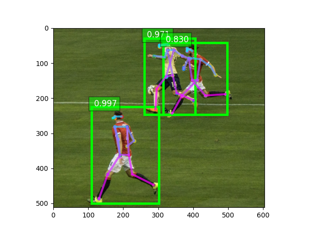
显示姿态估计结果

我们可以使用gluoncv.utils.viz.plot_keypoints()来可视化结果。

ax = utils.viz.plot_keypoints(img, pred_coords, confidence,
                              class_IDs, bounding_boxs, scores,
                              box_thresh=0.5, keypoint_thresh=0.2)
plt.show()