01. 使用预训练的 SSD 模型进行预测

本文将展示如何用少量代码使用预训练的 SSD 模型。

首先，让我们导入一些必要的库

from gluoncv import model_zoo, data, utils
from matplotlib import pyplot as plt

加载预训练模型

让我们获取一个在 Pascal VOC 数据集上使用 ResNet-50 V1 作为基础模型、并在 512x512 图像上训练的 SSD 模型。通过指定 pretrained=True，如果需要，它将自动从模型库下载模型。有关更多预训练模型，请参阅模型库。

net = model_zoo.get_model('ssd_512_resnet50_v1_voc', pretrained=True)

输出

/usr/local/lib/python3.6/dist-packages/mxnet/gluon/block.py:1512: UserWarning: Cannot decide type for the following arguments. Consider providing them as input:
        data: None
  input_sym_arg_type = in_param.infer_type()[0]
Downloading /root/.mxnet/models/ssd_512_resnet50_v1_voc-9c8b225a.zip from https://apache-mxnet.s3-accelerate.dualstack.amazonaws.com/gluon/models/ssd_512_resnet50_v1_voc-9c8b225a.zip...

  0%|          | 0/132723 [00:00<?, ?KB/s]
  0%|          | 102/132723 [00:00<02:50, 776.13KB/s]
  0%|          | 515/132723 [00:00<01:01, 2153.95KB/s]
  2%|1         | 2184/132723 [00:00<00:18, 6872.72KB/s]
  6%|5         | 7459/132723 [00:00<00:05, 21937.22KB/s]
 10%|9         | 13000/132723 [00:00<00:03, 32519.11KB/s]
 16%|#5        | 20998/132723 [00:00<00:02, 47353.06KB/s]
 21%|##        | 27272/132723 [00:00<00:02, 52010.10KB/s]
 26%|##5       | 34107/132723 [00:00<00:01, 57003.10KB/s]
 31%|###1      | 41248/132723 [00:01<00:01, 61167.62KB/s]
 37%|###6      | 48817/132723 [00:01<00:01, 65551.47KB/s]
 42%|####2     | 55878/132723 [00:01<00:01, 66907.14KB/s]
 48%|####7     | 63675/132723 [00:01<00:00, 70230.01KB/s]
 54%|#####3    | 71044/132723 [00:01<00:00, 71082.41KB/s]
 59%|#####9    | 78794/132723 [00:01<00:00, 73003.15KB/s]
 65%|######4   | 86212/132723 [00:01<00:00, 73073.51KB/s]
 71%|#######   | 93875/132723 [00:01<00:00, 74135.73KB/s]
 76%|#######6  | 101304/132723 [00:01<00:00, 73462.10KB/s]
 82%|########2 | 109276/132723 [00:01<00:00, 75321.61KB/s]
 88%|########8 | 116819/132723 [00:02<00:00, 73789.12KB/s]
 94%|#########4| 124842/132723 [00:02<00:00, 75683.59KB/s]
100%|#########9| 132424/132723 [00:02<00:00, 74238.46KB/s]
100%|##########| 132723/132723 [00:02<00:00, 59593.56KB/s]

预处理图像

接下来，我们下载一张图像，并使用预设的数据转换进行预处理。这里我们指定将图像的短边尺寸调整为 512 像素。但是您可以输入任意大小的图像。

如果您想同时加载多张图像，可以将图像文件名列表（例如 [im_fname1, im_fname2, ...]）提供给 gluoncv.data.transforms.presets.ssd.load_test()。

此函数返回两个结果。第一个是形状为 (batch_size, RGB_channels, height, width) 的 NDArray。它可以直接输入到模型中。第二个结果包含 numpy 格式的图像，方便绘制。由于我们只加载了一张图像，所以 x 的第一维是 1。

im_fname = utils.download('https://github.com/dmlc/web-data/blob/master/' +
                          'gluoncv/detection/street_small.jpg?raw=true',
                          path='street_small.jpg')
x, img = data.transforms.presets.ssd.load_test(im_fname, short=512)
print('Shape of pre-processed image:', x.shape)

输出

Downloading street_small.jpg from https://github.com/dmlc/web-data/blob/master/gluoncv/detection/street_small.jpg?raw=true...

  0%|          | 0/116 [00:00<?, ?KB/s]
117KB [00:00, 36875.08KB/s]
Shape of pre-processed image: (1, 3, 512, 512)

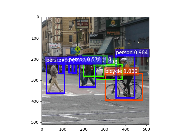
推理与显示

正向函数将返回所有检测到的边界框、相应的预测类别 ID 和置信度得分。它们的形状分别为 (batch_size, num_bboxes, 1)、(batch_size, num_bboxes, 1) 和 (batch_size, num_bboxes, 4)。

我们可以使用 gluoncv.utils.viz.plot_bbox() 来可视化结果。我们对第一张图像的结果进行切片，并将其输入到 plot_bbox 中。

class_IDs, scores, bounding_boxes = net(x)

ax = utils.viz.plot_bbox(img, bounding_boxes[0], scores[0],
                         class_IDs[0], class_names=net.classes)
plt.show()